All the Deep Learning Terms You Need to Know
Discussions: Hacker News (65 points, iv comments), Reddit r/MachineLearning (29 points, 3 comments)
Translations: Chinese (Simplified), French ane, French 2, Japanese, Korean, Russian, Spanish, Vietnamese
Watch: MIT's Deep Learning State of the Fine art lecture referencing this post
In the previous post, we looked at Attention – a ubiquitous method in mod deep learning models. Attention is a concept that helped improve the performance of neural automobile translation applications. In this post, we will look at The Transformer – a model that uses attention to boost the speed with which these models tin exist trained. The Transformer outperforms the Google Neural Machine Translation model in specific tasks. The biggest benefit, however, comes from how The Transformer lends itself to parallelization. Information technology is in fact Google Deject'southward recommendation to apply The Transformer equally a reference model to utilise their Cloud TPU offering. So let's try to break the model autonomously and expect at how information technology functions.
The Transformer was proposed in the paper Attending is All You lot Demand. A TensorFlow implementation of it is available as a role of the Tensor2Tensor package. Harvard'south NLP group created a guide annotating the newspaper with PyTorch implementation. In this post, nosotros volition attempt to oversimplify things a bit and introduce the concepts one by one to hopefully make it easier to understand to people without in-depth noesis of the discipline affair.
2020 Update: I've created a "Narrated Transformer" video which is a gentler approach to the topic:
A High-Level Look
Let's begin by looking at the model as a single black box. In a machine translation application, it would have a sentence in i linguistic communication, and output its translation in another.
![]()
Popping open that Optimus Prime goodness, we see an encoding component, a decoding component, and connections between them.
![]()
The encoding component is a stack of encoders (the paper stacks six of them on height of each other – in that location'southward naught magical about the number six, one tin can definitely experiment with other arrangements). The decoding component is a stack of decoders of the same number.
![]()
The encoders are all identical in structure (however they do not share weights). Each one is broken down into two sub-layers:
![]()
The encoder'southward inputs first flow through a cocky-attention layer – a layer that helps the encoder look at other words in the input sentence as it encodes a specific word. Nosotros'll look closer at self-attending later in the post.
The outputs of the self-attention layer are fed to a feed-forrad neural network. The exact same feed-forward network is independently practical to each position.
The decoder has both those layers, merely betwixt them is an attention layer that helps the decoder focus on relevant parts of the input sentence (like what attending does in seq2seq models).
![]()
Bringing The Tensors Into The Flick
Now that we've seen the major components of the model, let's outset to look at the various vectors/tensors and how they flow betwixt these components to turn the input of a trained model into an output.
As is the instance in NLP applications in full general, nosotros begin by turning each input word into a vector using an embedding algorithm.
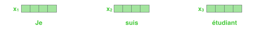
Each discussion is embedded into a vector of size 512. Nosotros'll represent those vectors with these simple boxes.
The embedding simply happens in the lesser-about encoder. The abstraction that is common to all the encoders is that they receive a listing of vectors each of the size 512 – In the bottom encoder that would be the word embeddings, but in other encoders, it would be the output of the encoder that'southward straight below. The size of this listing is hyperparameter we can set – basically it would be the length of the longest sentence in our training dataset.
Afterward embedding the words in our input sequence, each of them flows through each of the ii layers of the encoder.
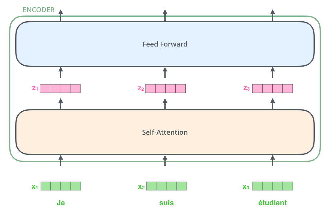
Hither nosotros brainstorm to come across one primal property of the Transformer, which is that the word in each position flows through its own path in the encoder. There are dependencies betwixt these paths in the self-attending layer. The feed-frontwards layer does not take those dependencies, still, and thus the diverse paths can be executed in parallel while flowing through the feed-forward layer.
Next, we'll switch upward the example to a shorter sentence and we'll look at what happens in each sub-layer of the encoder.
Now We're Encoding!
Every bit we've mentioned already, an encoder receives a list of vectors equally input. Information technology processes this listing by passing these vectors into a 'self-attention' layer, and so into a feed-forward neural network, then sends out the output upwards to the adjacent encoder.
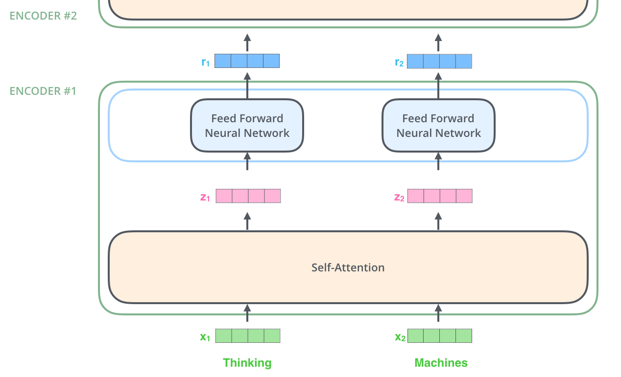
The word at each position passes through a self-attention process. And then, they each pass through a feed-forrard neural network -- the exact same network with each vector flowing through information technology separately.
Cocky-Attention at a High Level
Don't exist fooled by me throwing around the word "cocky-attention" like it's a concept anybody should exist familiar with. I had personally never came across the concept until reading the Attention is All Yous Demand paper. Permit u.s. dribble how it works.
Say the following judgement is an input sentence we want to translate:
"The animate being didn't cross the street because it was too tired"
What does "information technology" in this sentence refer to? Is it referring to the street or to the brute? Information technology's a simple question to a man, simply not as simple to an algorithm.
When the model is processing the word "information technology", self-attending allows it to associate "it" with "animate being".
As the model processes each discussion (each position in the input sequence), self attention allows information technology to look at other positions in the input sequence for clues that can help lead to a better encoding for this word.
If you're familiar with RNNs, think of how maintaining a hidden country allows an RNN to incorporate its representation of previous words/vectors it has processed with the electric current 1 information technology'south processing. Cocky-attending is the method the Transformer uses to bake the "understanding" of other relevant words into the one nosotros're currently processing.
![]()
As we are encoding the word "it" in encoder #5 (the top encoder in the stack), function of the attention mechanism was focusing on "The Animal", and baked a part of its representation into the encoding of "it".
Exist sure to check out the Tensor2Tensor notebook where y'all can load a Transformer model, and examine it using this interactive visualization.
Self-Attention in Detail
Let'south first wait at how to summate self-attention using vectors, then keep to look at how information technology's actually implemented – using matrices.
The offset pace in calculating self-attention is to create three vectors from each of the encoder'due south input vectors (in this case, the embedding of each word). So for each word, we create a Query vector, a Central vector, and a Value vector. These vectors are created by multiplying the embedding past three matrices that nosotros trained during the grooming procedure.
Notice that these new vectors are smaller in dimension than the embedding vector. Their dimensionality is 64, while the embedding and encoder input/output vectors have dimensionality of 512. They don't Accept to be smaller, this is an compages choice to brand the computation of multiheaded attention (mostly) constant.
![]()
Multiplying x1 past the WQ weight matrix produces q1, the "query" vector associated with that word. Nosotros end up creating a "query", a "key", and a "value" projection of each word in the input sentence.
What are the "query", "fundamental", and "value" vectors?
They're abstractions that are useful for computing and thinking virtually attention. Once you proceed with reading how attention is calculated below, you'll know pretty much all y'all need to know well-nigh the role each of these vectors plays.
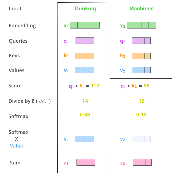
The 2nd step in computing self-attention is to summate a score. Say nosotros're calculating the self-attention for the first word in this case, "Thinking". We need to score each word of the input judgement against this word. The score determines how much focus to place on other parts of the input judgement as nosotros encode a word at a certain position.
The score is calculated by taking the dot product of the query vector with the key vector of the corresponding give-and-take we're scoring. So if we're processing the self-attention for the word in position #1, the first score would be the dot product of q1 and k1. The 2nd score would be the dot product of q1 and k2.
![]()
The third and 4th steps are to divide the scores by eight (the foursquare root of the dimension of the key vectors used in the paper – 64. This leads to having more stable gradients. At that place could exist other possible values here, merely this is the default), then laissez passer the outcome through a softmax functioning. Softmax normalizes the scores so they're all positive and add upwards to one.
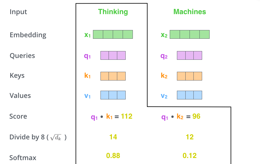
This softmax score determines how much each word will exist expressed at this position. Clearly the word at this position will have the highest softmax score, simply sometimes it's useful to attend to some other word that is relevant to the electric current word.
The fifth stride is to multiply each value vector past the softmax score (in preparation to sum them up). The intuition here is to keep intact the values of the give-and-take(s) we want to focus on, and drown-out irrelevant words (past multiplying them by tiny numbers like 0.001, for example).
The sixth step is to sum up the weighted value vectors. This produces the output of the self-attending layer at this position (for the get-go word).
That concludes the cocky-attending calculation. The resulting vector is one nosotros can send along to the feed-frontwards neural network. In the bodily implementation, however, this calculation is done in matrix class for faster processing. Then let's expect at that now that we've seen the intuition of the calculation on the word level.
Matrix Adding of Self-Attention
The starting time step is to calculate the Query, Primal, and Value matrices. Nosotros exercise that by packing our embeddings into a matrix 10, and multiplying it past the weight matrices we've trained (WQ, WK, WV).
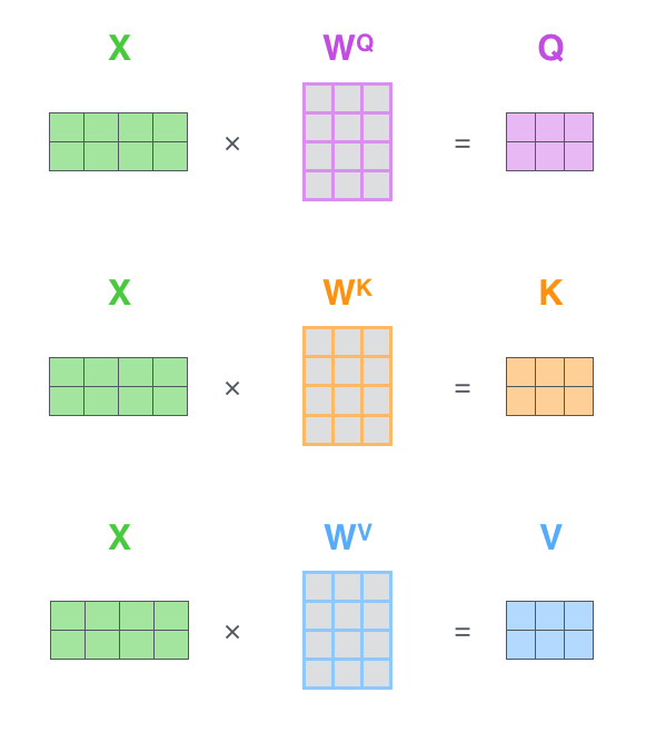
Every row in the X matrix corresponds to a word in the input judgement. We again run into the divergence in size of the embedding vector (512, or iv boxes in the figure), and the q/k/v vectors (64, or three boxes in the figure)
Finally, since nosotros're dealing with matrices, we can condense steps ii through six in ane formula to summate the outputs of the self-attention layer.
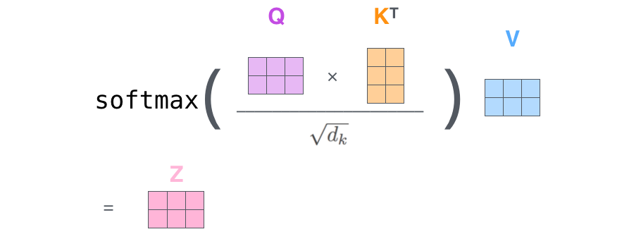
The cocky-attention adding in matrix form
The Beast With Many Heads
The paper further refined the cocky-attending layer by calculation a mechanism called "multi-headed" attending. This improves the functioning of the attending layer in two means:
-
Information technology expands the model's ability to focus on different positions. Yes, in the instance above, z1 contains a little bit of every other encoding, but information technology could be dominated by the the actual word itself. It would be useful if nosotros're translating a sentence like "The creature didn't cross the street considering it was too tired", we would want to know which word "it" refers to.
-
It gives the attention layer multiple "representation subspaces". As nosotros'll see adjacent, with multi-headed attending we have non only one, just multiple sets of Query/Key/Value weight matrices (the Transformer uses 8 attending heads, so we end up with viii sets for each encoder/decoder). Each of these sets is randomly initialized. Then, after training, each set is used to project the input embeddings (or vectors from lower encoders/decoders) into a different representation subspace.
![]()
With multi-headed attending, nosotros maintain separate Q/Grand/Five weight matrices for each head resulting in unlike Q/K/5 matrices. Equally we did before, we multiply X past the WQ/WK/WV matrices to produce Q/K/V matrices.
If nosotros do the same cocky-attending calculation we outlined above, just eight different times with different weight matrices, nosotros terminate upwardly with eight different Z matrices
![]()
This leaves united states with a bit of a challenge. The feed-forrard layer is not expecting eight matrices – it's expecting a single matrix (a vector for each discussion). So we demand a mode to condense these eight down into a single matrix.
How practice we practice that? We concat the matrices then multiply them past an boosted weights matrix WO.
![]()
That's pretty much all there is to multi-headed self-attention. It'due south quite a handful of matrices, I realize. Permit me try to put them all in ane visual and then we tin can look at them in 1 place
![]()
Now that we take touched upon attention heads, permit'southward revisit our example from before to run into where the different attention heads are focusing as we encode the discussion "information technology" in our example sentence:
![]()
As we encode the word "it", one attention caput is focusing near on "the animate being", while some other is focusing on "tired" -- in a sense, the model's representation of the word "it" bakes in some of the representation of both "animal" and "tired".
If we add together all the attention heads to the moving picture, however, things can be harder to translate:
![]()
Representing The Social club of The Sequence Using Positional Encoding
One thing that's missing from the model as we have described it and then far is a mode to account for the order of the words in the input sequence.
To address this, the transformer adds a vector to each input embedding. These vectors follow a specific design that the model learns, which helps it determine the position of each discussion, or the distance between different words in the sequence. The intuition here is that adding these values to the embeddings provides meaningful distances between the embedding vectors one time they're projected into Q/K/V vectors and during dot-product attention.
![]()
To give the model a sense of the order of the words, nosotros add positional encoding vectors -- the values of which follow a specific pattern.
If we causeless the embedding has a dimensionality of 4, the actual positional encodings would look similar this:
![]()
A real example of positional encoding with a toy embedding size of 4
What might this design expect like?
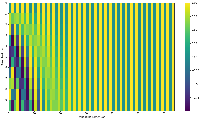
In the post-obit effigy, each row corresponds to a positional encoding of a vector. So the kickoff row would be the vector we'd add to the embedding of the showtime word in an input sequence. Each row contains 512 values – each with a value between 1 and -1. We've color-coded them and then the design is visible.
![]()
A existent instance of positional encoding for 20 words (rows) with an embedding size of 512 (columns). You tin can see that it appears carve up in half downwardly the centre. That's considering the values of the left half are generated past one function (which uses sine), and the right half is generated by another function (which uses cosine). They're then concatenated to form each of the positional encoding vectors.
The formula for positional encoding is described in the newspaper (section 3.5). You tin can meet the code for generating positional encodings in get_timing_signal_1d(). This is non the but possible method for positional encoding. It, however, gives the reward of existence able to scale to unseen lengths of sequences (e.1000. if our trained model is asked to interpret a sentence longer than any of those in our grooming set).
July 2020 Update: The positional encoding shown above is from the Tranformer2Transformer implementation of the Transformer. The method shown in the newspaper is slightly different in that it doesn't directly concatenate, but interweaves the ii signals. The following figure shows what that looks like. Here'south the code to generate it:
The Residuals
One particular in the compages of the encoder that we need to mention before moving on, is that each sub-layer (cocky-attention, ffnn) in each encoder has a residual connectedness effectually it, and is followed past a layer-normalization step.
![]()
If we're to visualize the vectors and the layer-norm operation associated with self attending, it would wait like this:
![]()
This goes for the sub-layers of the decoder as well. If nosotros're to recall of a Transformer of 2 stacked encoders and decoders, it would look something similar this:
![]()
The Decoder Side
Now that we've covered well-nigh of the concepts on the encoder side, we basically know how the components of decoders work too. But allow's take a await at how they work together.
The encoder kickoff past processing the input sequence. The output of the top encoder is so transformed into a set of attending vectors G and 5. These are to be used by each decoder in its "encoder-decoder attention" layer which helps the decoder focus on appropriate places in the input sequence:
![]()
Later on finishing the encoding phase, nosotros begin the decoding stage. Each pace in the decoding stage outputs an element from the output sequence (the English translation judgement in this case).
The following steps repeat the process until a special
![]()
The self attention layers in the decoder operate in a slightly different fashion than the one in the encoder:
In the decoder, the self-attention layer is just immune to nourish to earlier positions in the output sequence. This is washed past masking future positions (setting them to -inf) before the softmax stride in the self-attending calculation.
The "Encoder-Decoder Attention" layer works just similar multiheaded self-attending, except it creates its Queries matrix from the layer below it, and takes the Keys and Values matrix from the output of the encoder stack.
The Last Linear and Softmax Layer
The decoder stack outputs a vector of floats. How do we plow that into a word? That'southward the job of the last Linear layer which is followed by a Softmax Layer.
The Linear layer is a simple fully connected neural network that projects the vector produced past the stack of decoders, into a much, much larger vector called a logits vector.
Let'south assume that our model knows 10,000 unique English words (our model's "output vocabulary") that it'south learned from its training dataset. This would make the logits vector 10,000 cells wide – each cell corresponding to the score of a unique discussion. That is how we interpret the output of the model followed by the Linear layer.
The softmax layer then turns those scores into probabilities (all positive, all add up to 1.0). The cell with the highest probability is chosen, and the word associated with it is produced every bit the output for this time footstep.
![]()
This figure starts from the bottom with the vector produced as the output of the decoder stack. It is then turned into an output give-and-take.
Recap Of Grooming
At present that we've covered the entire forward-pass procedure through a trained Transformer, information technology would exist useful to glance at the intuition of training the model.
During preparation, an untrained model would become through the exact same forwards pass. But since nosotros are grooming it on a labeled preparation dataset, nosotros can compare its output with the actual correct output.
To visualize this, permit'due south assume our output vocabulary only contains six words("a", "am", "i", "thanks", "educatee", and "<eos>" (curt for 'cease of sentence')).
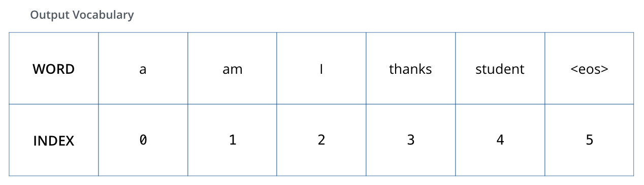
The output vocabulary of our model is created in the preprocessing phase before we even brainstorm preparation.
Once nosotros ascertain our output vocabulary, nosotros tin can utilize a vector of the same width to indicate each word in our vocabulary. This besides known every bit one-hot encoding. Then for example, we tin signal the word "am" using the following vector:
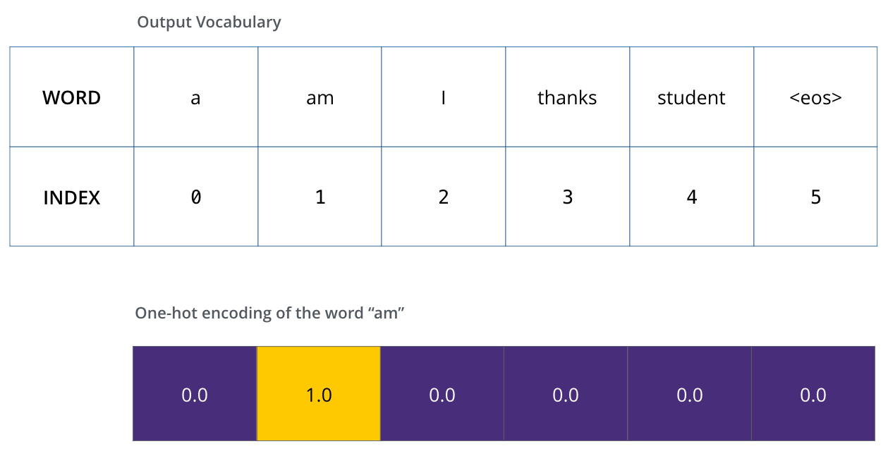
Example: one-hot encoding of our output vocabulary
Following this epitomize, allow's discuss the model'southward loss function – the metric we are optimizing during the grooming phase to lead upward to a trained and hopefully amazingly authentic model.
The Loss Function
Say we are preparation our model. Say information technology's our get-go step in the training phase, and we're training it on a elementary example – translating "merci" into "thank you".
What this means, is that we want the output to exist a probability distribution indicating the give-and-take "thank you". But since this model is not yet trained, that'south unlikely to happen only yet.
![]()
Since the model's parameters (weights) are all initialized randomly, the (untrained) model produces a probability distribution with arbitrary values for each cell/give-and-take. We can compare it with the actual output, so tweak all the model'southward weights using backpropagation to make the output closer to the desired output.
How do you compare two probability distributions? We simply subtract one from the other. For more details, look at cross-entropy and Kullback–Leibler departure.
Only note that this is an oversimplified example. More than realistically, we'll use a sentence longer than one word. For example – input: "je suis étudiant" and expected output: "i am a student". What this really means, is that we want our model to successively output probability distributions where:
- Each probability distribution is represented by a vector of width vocab_size (vi in our toy instance, but more realistically a number like 30,000 or 50,000)
- The start probability distribution has the highest probability at the prison cell associated with the discussion "i"
- The second probability distribution has the highest probability at the cell associated with the give-and-take "am"
- And and then on, until the 5th output distribution indicates '
<finish of sentence>' symbol, which as well has a cell associated with information technology from the 10,000 element vocabulary.
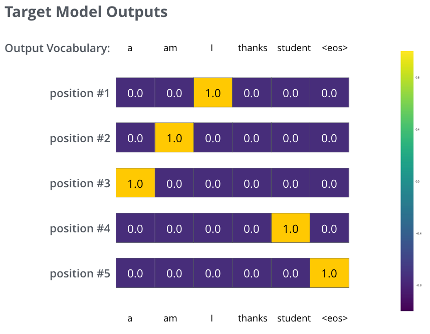
The targeted probability distributions we'll railroad train our model against in the preparation example for ane sample sentence.
After preparation the model for enough fourth dimension on a large enough dataset, we would promise the produced probability distributions would await similar this:
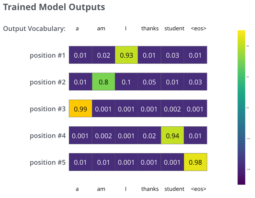
Hopefully upon grooming, the model would output the correct translation we expect. Of form it'south no existent indication if this phrase was role of the training dataset (see: cross validation). Notice that every position gets a little scrap of probability fifty-fifty if it's unlikely to be the output of that fourth dimension step -- that's a very useful property of softmax which helps the training process.
Now, considering the model produces the outputs one at a time, we can assume that the model is selecting the word with the highest probability from that probability distribution and throwing abroad the rest. That's i style to do it (chosen greedy decoding). Another manner to practise information technology would be to agree on to, say, the elevation two words (say, 'I' and 'a' for example), so in the next footstep, run the model twice: once assuming the first output position was the word 'I', and another fourth dimension bold the start output position was the word 'a', and whichever version produced less error considering both positions #ane and #2 is kept. We repeat this for positions #2 and #3…etc. This method is called "beam search", where in our example, beam_size was 2 (meaning that at all times, two partial hypotheses (unfinished translations) are kept in retentiveness), and top_beams is also two (meaning we'll return two translations). These are both hyperparameters that y'all can experiment with.
Go Forth And Transform
I hope you've establish this a useful place to commencement to break the ice with the major concepts of the Transformer. If you desire to go deeper, I'd propose these next steps:
- Read the Attention Is All Y'all Need newspaper, the Transformer blog post (Transformer: A Novel Neural Network Architecture for Linguistic communication Understanding), and the Tensor2Tensor annunciation.
- Watch Łukasz Kaiser'southward talk walking through the model and its details
- Play with the Jupyter Notebook provided every bit office of the Tensor2Tensor repo
- Explore the Tensor2Tensor repo.
Follow-up works:
- Depthwise Separable Convolutions for Neural Auto Translation
- One Model To Larn Them All
- Detached Autoencoders for Sequence Models
- Generating Wikipedia by Summarizing Long Sequences
- Paradigm Transformer
- Training Tips for the Transformer Model
- Cocky-Attention with Relative Position Representations
- Fast Decoding in Sequence Models using Discrete Latent Variables
- Adafactor: Adaptive Learning Rates with Sublinear Retention Cost
Acknowledgements
Thanks to Illia Polosukhin, Jakob Uszkoreit, Llion Jones , Lukasz Kaiser, Niki Parmar, and Noam Shazeer for providing feedback on earlier versions of this mail.
Please hit me up on Twitter for whatsoever corrections or feedback.
Source: https://jalammar.github.io/illustrated-transformer/
0 Response to "All the Deep Learning Terms You Need to Know"
Post a Comment